We use the statistical model of aftershock rate developed by Reasenberg and Jones (1989, 1994). In this model, the rate R of aftershocks of at least magnitude M, at time T after a magnitude Mmain mainshock, is:
Equation 1: $$\text{R} = 10^{\text{a} + \text{b} (\text{Mmain} - \text{M}))} (\text{T} + \text{c}) ^ {(-\text{p})}$$
where a, b, c, and p are model parameters. The parameter a represents the regional aftershock productivity, b represents the scaling of aftershock rate with mainshock magnitude, p represents the decay of the rate of aftershocks with time, and c is the time scale of the earliest part of the sequence before it starts to decay. Reasenberg and Jones (1989) found values of these parameters for California aftershock sequences, and Hardebeck et al. (2018) updated these parameters with more modern data and finer regionalization.
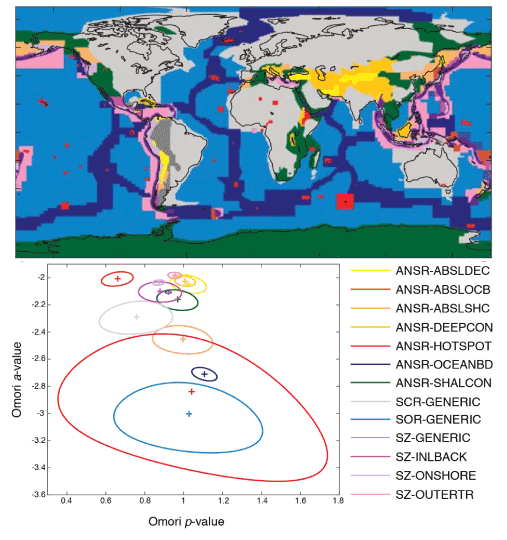
Page et al. (2016) extended the Reasenberg and Jones (1989) method to apply globally by grouping tectonically similar areas together, using the tectonic regionalization of García et al. (2012), and determining parameter values for each global tectonic regime. Page et al. (2016) also found the productivity parameter a for each mainshock in each tectonic regime, and described the collection of a-values with a normal distribution. This distribution is used to generate forecasts with uncertainty bounds that reflect the parameter uncertainty, as well as random variability. Page et al. (2016) further improved upon the Reasenberg and Jones (1989) method by better accounting for smaller aftershocks that may be missing from the catalog in the early part of the aftershock sequence when there are too many earthquakes occurring to locate all of them.

The Reasenberg and Jones (1989) model assumes all aftershocks are triggered by the mainshock, which is not always an accurate assumption. It works well for mainshocks followed only by smaller aftershocks, but may perform poorly for sequences with large aftershocks that trigger many of their own aftershocks. It also may perform poorly for swarms of multiple similar-sized earthquakes, which may be driven by fluid-flow or slow slip. Future versions of this product will address these limitations of the Reasenberg and Jones (1989) model.
Generic Model Parameters
Generic forecasts are computed using the “generic” model parameters for the earthquake’s tectonic regime. For most events, the generic parameter values are those from Page et al. (2016). For events in California, the generic parameter values are from Hardebeck et al. (2018).
The generic model parameters include substantial uncertainty, due to the variability in behavior of previously observed aftershock sequences, so the generic aftershock forecasts also tend to have large uncertainty. The parameter uncertainty is expressed in Page et al. (2016) and Hardebeck et al. (2018) as uncertainty in the productivity parameter a, and quantified as a normal probability distribution function for the a-value, denoted Pgeneric(a).
The forecast for a given magnitude range and time period is computed by constructing a probability distribution for the number N of aftershocks, P(N). We discretize the a-value probability distribution, Pgeneric(a), and for each a-value, ai, we compute the corresponding number of aftershocks, Ni. We find Ni by putting ai and the fixed values of b, p, and c into Equation 1 and integrating over the given time period. We next account for random variability by generating a Poisson distribution with a mean of Ni, Pi(N), which is the probability distribution for the number of aftershocks assuming an a-value of ai. We then sum these distributions, weighted by the probability of the corresponding a-value:
Equation 2: $$\text{P}(\text{N}) = \sum_i[\text{P}_i(\text{N}) * \text{P}_\text{generic}(\text{a}_i)]$$
We then use the probability distribution for the number of aftershocks, P(N), to compute the forecast. The probability of at least one aftershock in the given magnitude range and time period is the complement of the probability of zero aftershocks, so prob(N≥1)=1-P(0). The likely number of aftershocks is given as the 95% confidence range, Nmin to Nmax, where prob(N≤Nmin)≈0.025 and prob(N≤Nmax)≈0.975 (the equalities are approximate due to the inherent discreteness of the P(N) distribution).
Sequence-Specific Model Parameters
The sequence-specific model parameters are computed from the aftershocks that have been observed up to the time of the forecast. Usually, we retain the generic values of b, p, and c, and determine a sequence-specific value for just for the productivity a-value. It has been shown that fitting more than one parameter for a single sequence can be unstable (Llenos and Michael, 2017). For sequences with an unusually high or low rate of decay with time, we may also fit a sequence-specific p-value.
We determine the a-value (and possibly the p-value) by finding the value that maximizes the likelihood, L, of observing the actual aftershocks given the model and parameter values. We use the likelihood equation given by Ogata (1983). We find the likelihood for the discretized values of a, L(a). The likelihood scales with the probability that the parameter values are correct, so we can use the likelihood to define the sequence-specific probability distribution function for the a-value,
Equation 3: $$\text{P}_{seq-spec}(\text{a}) = \frac{L(\text{a})}{(\sum_i\text{L}(\text{a}i))}$$. The probability distribution for the number of aftershocks, P(N), and the forecast can then be computed using the same procedures as for the generic model, using Pseq-spec(a) instead of Pgeneric(a).
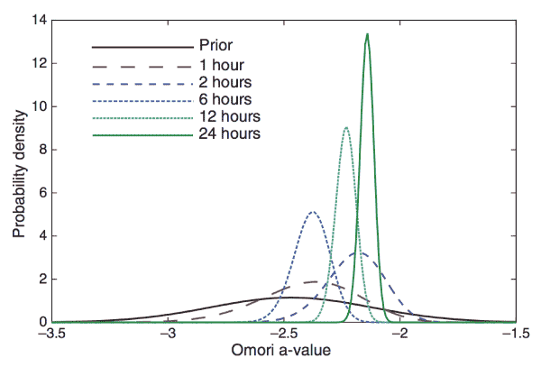
Using the sequence-specific parameters usually reduces the uncertainty of the forecast, compared to the generic parameters, because it ignores the observed variability of prior sequences. Because it neglects this variability, it is possible that the sequence-specific parameters may reduce the uncertainty too much. This problem is addressed by the Bayesian model parameters, which are generally preferred over the sequence-specific parameters.
Bayesian Model Parameters
The Bayesian model updates the generic parameters using the observed aftershock sequence up to the time of the forecast. The generic probability distribution function for the a-value, Pgeneric(a), is used as the Bayesian prior. Following Bayes’ theorem, the prior is multiplied by the likelihood of observing the data given the parameter values to compute the posterior distribution, in this case PBayes(a) = Pgeneric(a)* L(a), normalized such that the total probability is 1. The probability distribution for the number of aftershocks, P(N), and the forecast are computed using the same procedure as for the generic model, using PBayes(a) instead of Pgeneric(a). The Bayesian model only differs from the generic model when the observations force it to. Therefore, the Bayesian model resembles the generic model early in the sequence, and transitions to resembling the sequence-specific model later in the sequence.

References
- García, D., D. J. Wald, and M. G. Hearne (2012). A global earthquake discrimination scheme to optimize ground-motion prediction equation selection, Bulletin of the Seismological Society of America, vol. 102, pp. 185–203.
- Hardebeck J.L, A.L. Llenos, A.J. Michael, M.T. Page and N. van der Elst. (2018). Updated California Aftershock Parameters, Seismological Research Letters, vol. 90, pp. 262-270.
- Llenos, A. L., and A. J. Michael (2017). Forecasting the (un)productivity of the 2014 M 6.0 South Napa aftershock sequence, Seismological Research Letters, vol. 88, pp. 1241-1251.
- Ogata, Y. (1983). Estimation of the parameters in the modified Omori formula for aftershock frequencies by the maximum likelihood procedure, Journal of Physics of the Earth, vol. 31(2), pp. 115-124.
- Page, M. T., N. Van Der Elst, J. Hardebeck, K. Felzer, and A. J. Michael (2016). Three ingredients for improved global aftershock forecasts: Tectonic region, time-dependent catalog incompleteness, and intersequence variability, Bulletin of the Seismological Society of America, vol. 106, pp. 2290-2301.
- Reasenberg, P. A., and L. M. Jones (1989). Earthquake hazard after a mainshock in California, Science, vol. 243, pp. 1173–1176.
- Reasenberg, P. A., and L. M. Jones (1994). Earthquake aftershocks: update, Science, vol. 265, pp. 1251-1253.
 Jump to Navigation