Earthquake-triggered landslides and liquefaction, collectively referred to as ground failure, can be a significant contributor to earthquake losses. The USGS Ground Failure (GF) earthquake product provides near-real-time spatial estimates of earthquake-triggered landslide and liquefaction hazard following significant earthquakes worldwide.
We developed this product to provide initial awareness of the overall extent and importance of potential landslides and liquefaction, and to indicate areas in which they are most likely to have occurred. It takes time for first responders and experts to survey the actual damage in the area, so our product provides early estimates of where to focus attention and response planning. Though our models provide regional estimates of landslide and liquefaction hazard triggered by this earthquake, they do not predict specific occurrences.
The GF product is based on a suite of geospatial models that relate ground motion estimates provided by the USGS ShakeMap and proxies for ground failure susceptibility to rapidly provide regional estimates of earthquake-triggered ground failure hazard over a grid of evenly-spaced points. The GF product is summarized below. Refer to Allstadt and others (2022) for the full technical details.
Product Overview
Triggering
The creation of a USGS ShakeMap triggers the GF product under two conditions:
- Magnitude of M4.5 or greater and a maximum peak ground acceleration (PGA) of 10% g.
- Magnitude of M6.0 or greater.
Results are always shown if the GF product is run, even for events for which little to no ground failure is estimated.
Product Card
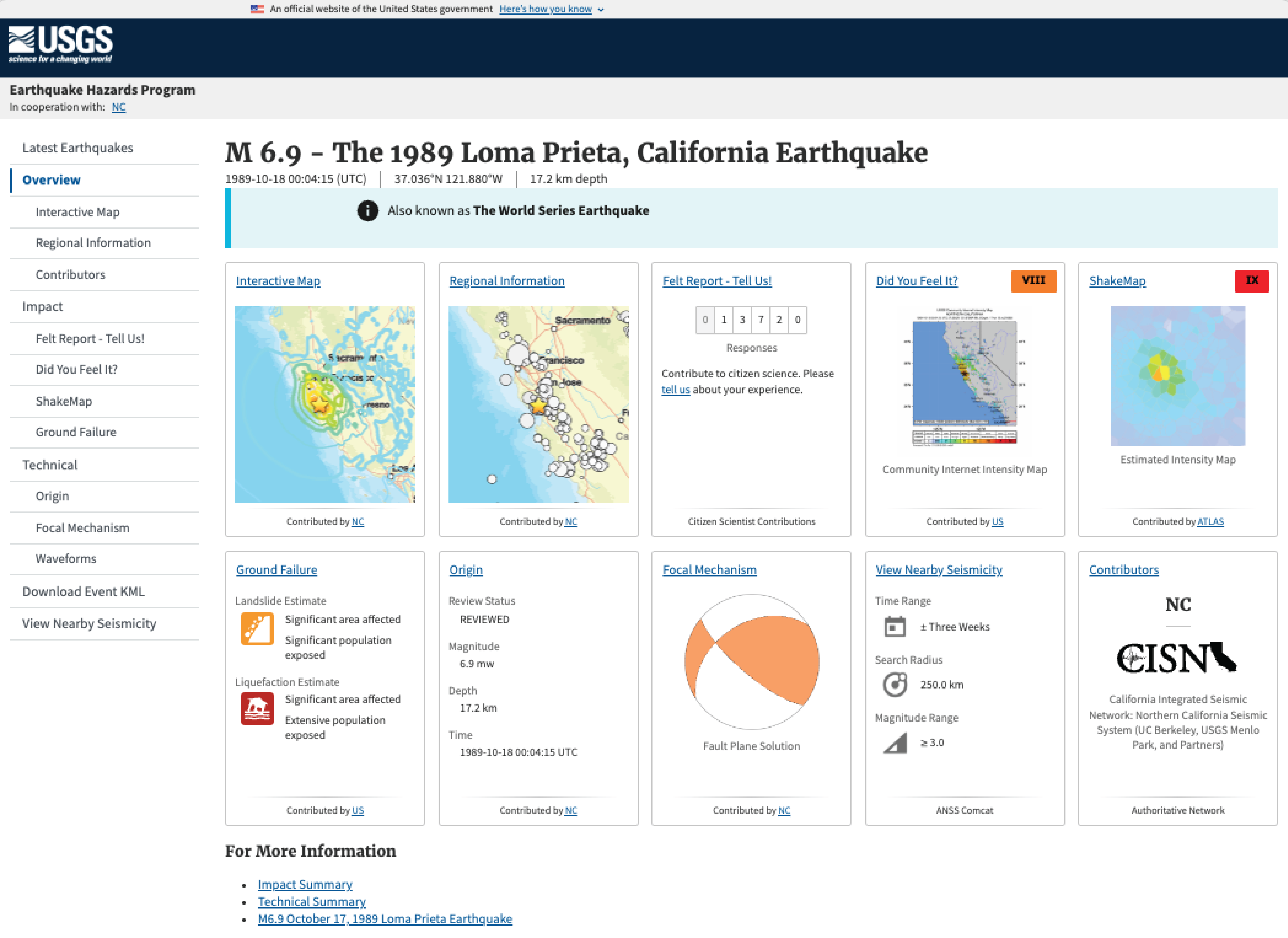
Ground Failure is considered a new earthquake information product, one of the suite of USGS Earthquake Program information systems that provide situational awareness and scientific content pertaining to each significant earthquake around the globe. The user will typically navigate to the Ground Failure page for a specific earthquake by starting at the overview of the earthquake-specific webpage (Figure 1) and selecting the card titled “Ground Failure.” This card will only appear if GF was triggered (see above). The card summarizes the landslide and liquefaction hazard for this event qualitatively (e.g., significant area affected, extensive population exposed). The color of the icon next to each ground failure type corresponds to the maximum of the two alert levels.
Summary Page
Selecting the Ground Failure card takes the user to the Summary page for Ground Failure. This page gives the user an overview of the hazard and population exposure for the two different types of ground failure and allows the user to navigate to interactive maps and other features, as described in the following sections and labeled in Figure 2.
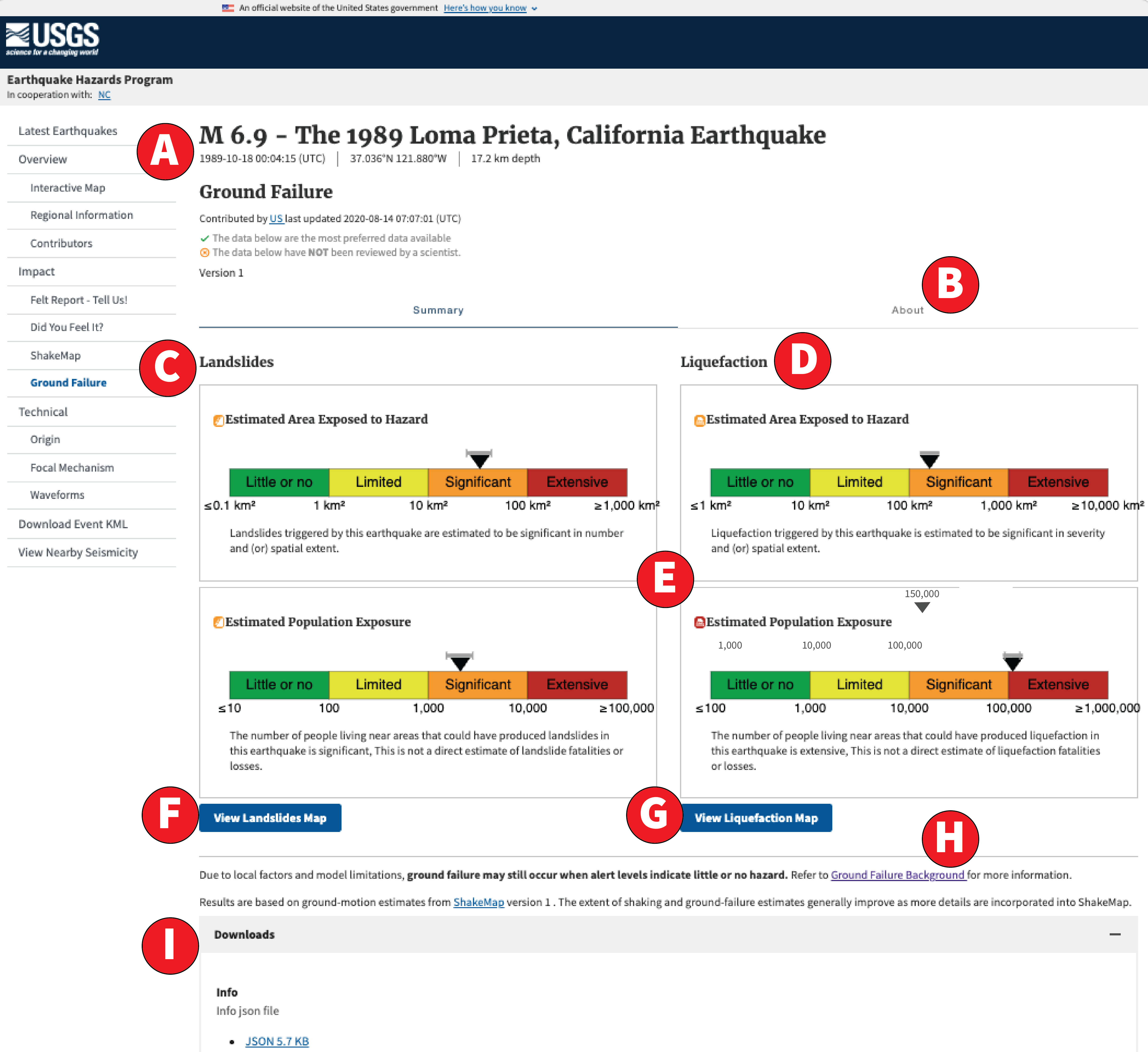
A) Earthquake Summary
The top of all earthquake event webpages consists of a summary of the most up-to-date earthquake information (magnitude, geographic location, event time, and epicentral location). Below this is the title of the product and time of last update.
B) "About" Tab
This tab provides basic information for the general public that describes why we developed this product, how to use it, what earthquake-triggered landslides and liquefaction are, and what hazards they pose to human populations. The simplified information provided in this tab is intended for non-expert users who may not be interested in the level of detail provided on this detailed webpage.
C, D) Landslide and Liquefaction Models
The left column of the summary webpage summarizes the landslide hazard and exposure alert levels for this earthquake based on our preferred landslide model, and the right column corresponds to the same for liquefaction. On mobile devices, these columns will be stacked on top of each other.
E) Alert Levels
The four alert level bars on the Ground Failure summary webpage give a quick overview of the expected hazard and population exposure for each ground failure type (Figure 3).
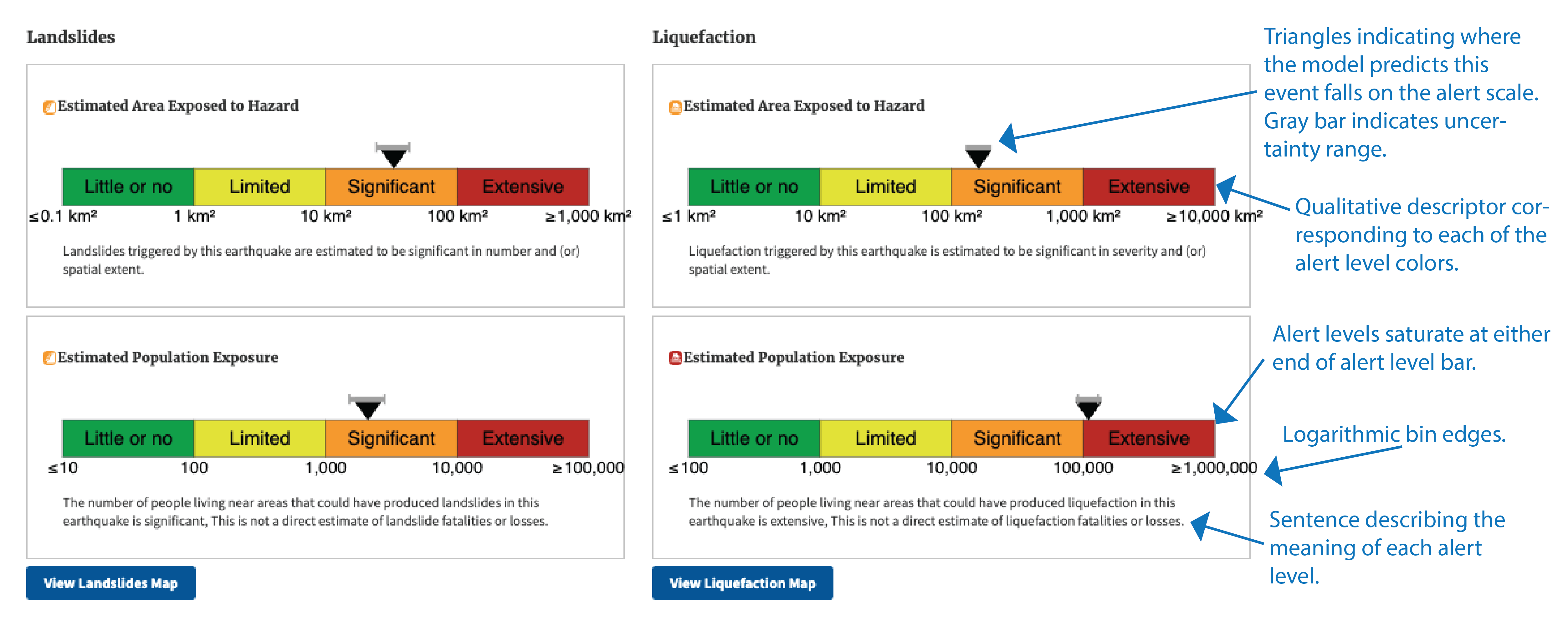
The alert levels are determined using two statistical parameters for each model type: Estimated Area Exposed to Hazard (Htot) and Estimated Population Exposure (popexp). (Htot) is equivalent to the model's estimate of the total area exposed to hazard in km2, and popexp is the approximate number of people who live in the areas exposed to hazard. See the Statistics section for details about how these are computed.
The alert level bins are each defined by a qualitative order-of-magnitude range for each statistic, which were chosen based on historic earthquakes with known consequences. See the Alert Level Definitions section for details.
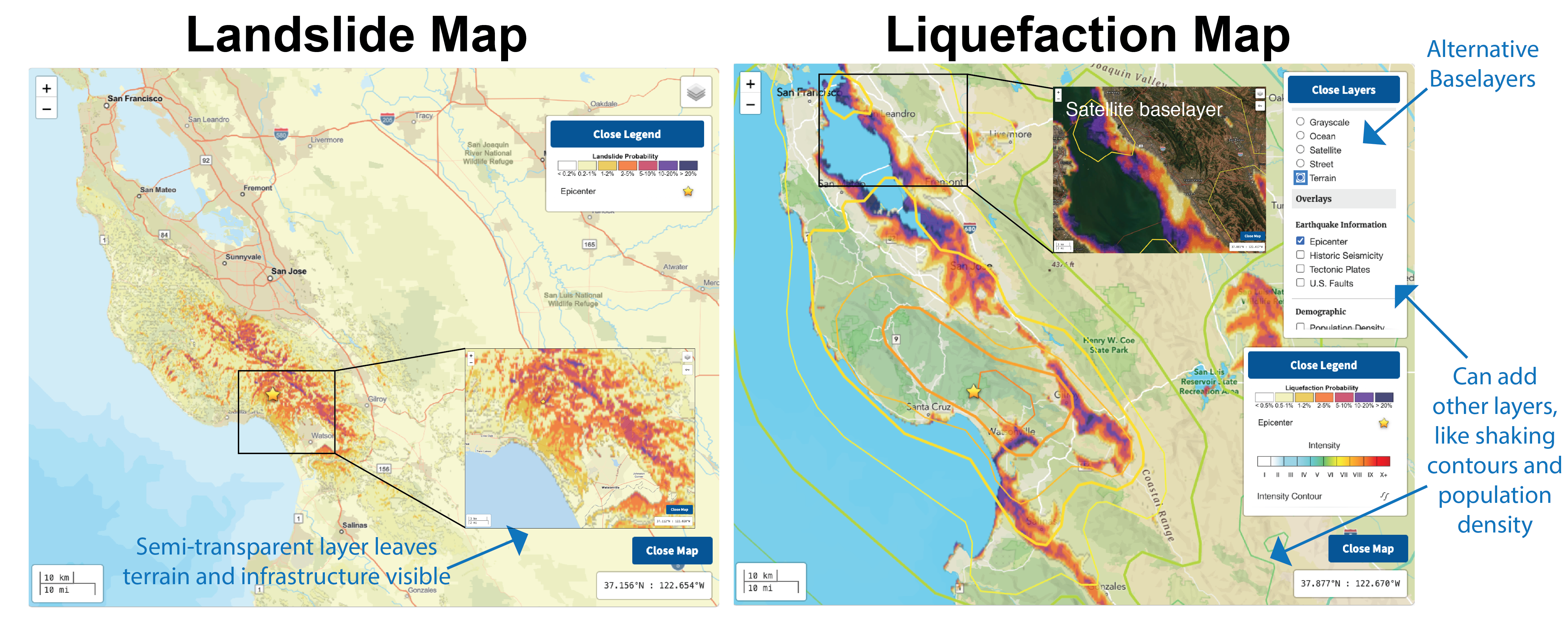
F, G) Interactive Map
Selecting the “View Landslide Map” button takes the user to the interactive map with the preferred landslide model shown by default. The same applies to the “View Liquefaction Map” button. The interactive map includes numerous alternative basemap layers and earthquake layers that can be superimposed on the landslide or liquefaction hazard maps (Figure 4). The colorbars for both landslides and liquefaction (Figure 5) show the areal coverage probability type (see Interpretation of Maps) using logarithmic bins to better visualize the range of typical values. The colorbar saturates at 0.2, which for areal coverage, equates to severe ground failure. Neither model reaches values much higher than 0.2 for areal coverage. Probabilities are never exactly zero for logistic models, but we mask areas with insignificant probabilities on the interactive maps, as indicated by the lower bound of the color bars (Figure 5).
H) Ground Failure Background Page
A footer appears at the bottom of all Ground Failure product pages with basic disclaimers about the product and a link to a static webpage that provides detailed technical information for advanced users (this webpage).
Downloads
The Downloads expansion panel allows advanced users to download GIS files of all ground failure model results, including the alternative model results, which are not currently shown on the interactive map.
Models
The GF models are designed to be rapidly and consistently applicable in any region of the world, requiring that they be relatively simple and depend on globally-available input datasets. There are many factors that contribute to a given occurrence of ground failure that are unknowable at the global scale; thus the models are not able to account for local characteristics of topography or geology nor to predict specific occurrences.
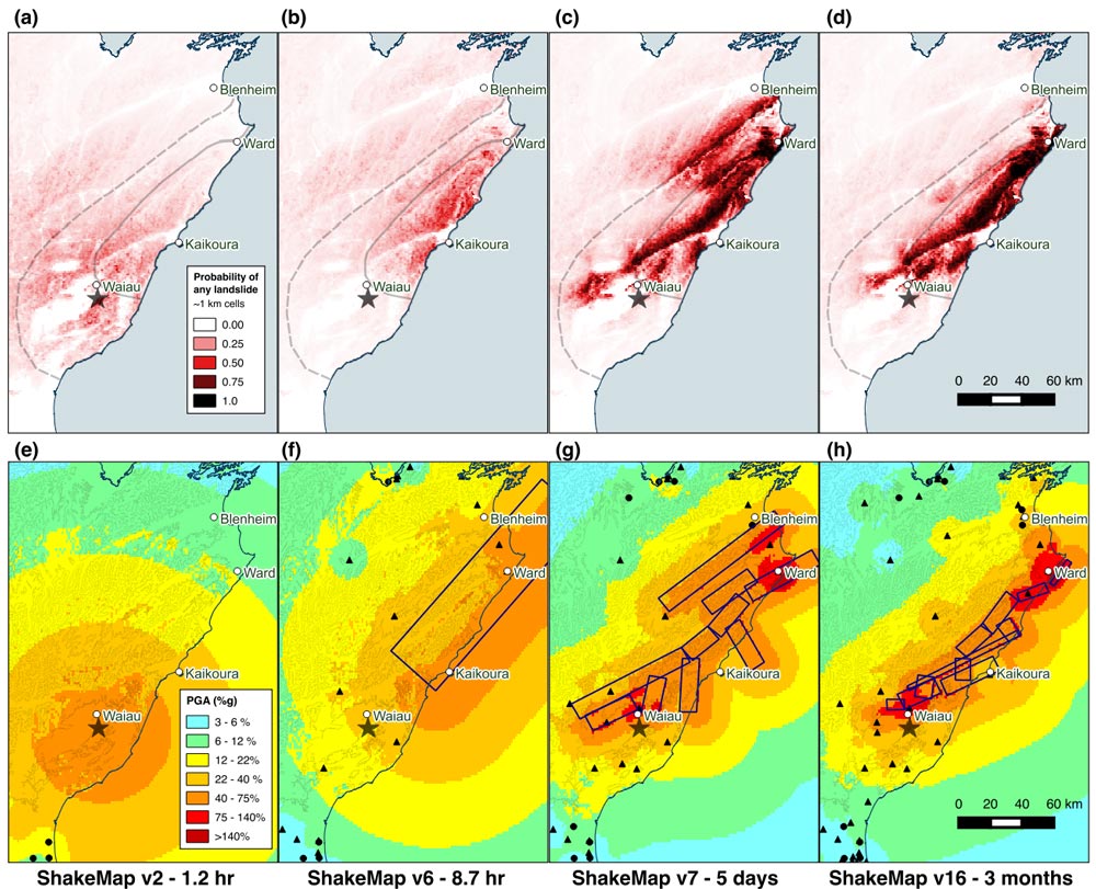
Although the models differ in detail, in general, they indicate that landsliding is more likely where shaking is strong and slopes are steep, and that liquefaction is more likely where shaking is strong and the land is flat and wet. The quality of the model outputs also depend, in part, on the quality of the ShakeMap estimates of ground motion. Model calibration was done using final ShakeMaps for about two dozen earthquakes. Thus, our estimates generally improve with time as observed shaking data and estimates of rupture extent are incorporated (Figure 6).
We currently use one preferred landslide model and one preferred liquefaction model for the product summary and interactive maps, but we also run several alternative models that are available for users to download. All implemented models are summarized below; details can be found in the original publications. For more detailed information on our implementation of these models, refer to the software release.
Preferred Landslide Model
Nowicki Jessee and others (2018) is the preferred model for earthquake-triggered landslide hazard. Our primary landslide model is the empirical model of Nowicki Jessee and others (2018). The model was developed by relating 23 inventories of landslides triggered by past earthquakes with different combinations of predictor variables (summarized below) using logistic regression. The output resolution is ~250 m. The model inputs are described below. More details about the model can be found in the original publication. We modify the published model by excluding areas with slopes <5° and changing the coefficient for the lithology layer "unconsolidated sediments" from -3.22 to -1.36, the coefficient for "mixed sedimentary rocks" to better reflect that this unit is expected to be weak (more negative coefficient indicates stronger rock).To exclude areas of insignificantly small probabilities in the computation of aggregate statistics for this model, we use a probability threshold of 0.002.
Table 1: Summary of Nowicki Jessee and others (2018) model inputs
| Input | Source |
|---|---|
| Slope | Derived from Global Multi-resolution Terrain Elevation Data 2010 (GMTED2010) (Danielson and Gesch, 2011) |
| Peak Ground Velocity (PGV) | U.S. Geological Survey ShakeMap (Worden and Wald, 2016) |
| Lithology | Global Lithological Map Database (GLiM) (Hartmann and Moosdorf, 2012) |
| Land cover | Moderate resolution (300 m) Envisat MERIS (MEdium Resolution Imaging Spectrometer) GlobCover land cover dataset for 2009 (Arino and others, 2012) |
| Compound topographic index (CTI) (wetness index) | U.S. Geological Survey HYDRO1k geographic database (Moore and others, 1991) |
Preferred Liquefaction Model
Zhu and others (2017) is the preferred model for liquefaction hazard. The model was developed by relating 27 inventories of liquefaction triggered by past earthquakes to globally-available geospatial proxies (summarized below) using logistic regression. We have implemented the global version of the model and have added additional modifications proposed by Baise and Rashidian (2017), including a peak ground acceleration (PGA) threshold of 0.1 g and linear interpolation of the input layers. We also exclude areas with slopes >5°. We linearly interpolate the original input layers of ~1 km resolution to 500 m resolution. The model inputs are described below. More details about the model can be found in the original publication.
Table 2: Summary of Zhu and others (2017) model inputs
| Input | Source |
|---|---|
| Peak Ground Velocity (PGV) | U.S. Geological Survey ShakeMap (Worden and Wald, 2016) |
| Shear wave velocity averaged over top 30 m (Vs30) | Computed from GMTED2010 using methods of Wald and Allen (2007) based on topographic slope |
| Mean Annual Precipitation | WorldClim database, last accessed March 2014 (Hijmans and others, 2005) |
| Distance from coast | Global distance to coast dataset by NASA's Ocean Color Group |
| Distance from rivers | Computed from U.S. Geological Survey HydroSHEDS database |
| Water table depth | Global model by Fan and others (2013) |
Our initial testing of the Zhu and others (2017) model indicated that some moderate magnitude events were over predicting liquefaction probabilities. Thus, we applied the following ad-hoc equation to mitigate this problem:
$$\text{SF} = \frac{1}{1 + \exp(-2[M - 6])}$$
where M is the earthquake magnitude. We multiply PGV by SF before it is evaluated in the Zhu and others (2017) model. This is analogous to how the Youd and others (2001) magnitude scaling factor works for PGA, except that it is applied to PGV, and we compare the two in Figure 7. Note that we are showing
Alternative Models
We currently run two alternative landslide models and one alternative liquefaction model, described in Table 3. These models are not currently rendered on the interactive map or used to determine alert levels, but are available for download.
Table 3: Summary of Alternative Models
| Type | Model Name | Input Layers | Resolution |
|---|---|---|---|
| Landslide | Nowicki and others (2014) | Maximum slope (~90 m resolution), Peak Ground Acceleration, Friction angle, Compound topographic index (wetness proxy) | ~1 km |
| Landslide | Godt and others (2008) | Slope quantiles (~1 km resolution derived from ~90 m resolution), Peak Ground Acceleration, Cohesion, Friction angle | ~1 km |
| Liquefaction | Zhu and others (2015) | Peak Ground Acceleration, Shear wave velocity averaged over top 30 m (Vs30), Compound topographic index | ~1 km |
Interpretation of Maps
Both of our preferred models are logistic models. Logistic models estimate probability, but the meaning of that probability depends on how the model was developed. The methods of our preferred models (Nowicki Jessee and others 2018 and Zhu and others 2017) result in a native output of relative hazard. This does not have a physical meaning. Therefore, both authors calibrated their models against completely mapped inventories to develop a relation to convert relative hazard to a different type of probability that does have a physical meaning: areal coverage (Ac). The meaning of Ac is illustrated in Figure 8.
The Godt and others (2008) and Zhu and others (2015) models both estimate areal coverage natively without requiring a conversion. The Nowicki and others (2014) model is distinct from the others in that it estimates the probability of any landslide occurring within a given grid cell.
Statistics
Statistical parameters used to summarize the model results and to assign hazard and population exposure alert levels are Estimated Area Exposed to Hazard (Htot), and population exposure (popexp). We use a ground motion threshold of 0.1g to compute these statistics in order to control for differences in the ShakeMap areas between events. The spatial extent of the ShakeMap can vary substantially from event to event and even for subsequent versions of the same event, and this can have an artificial impact on the statistics if not controlled for. Using a ground motion threshold also helps mitigate the inflation of these statistics due to small probabilities over large areas by only considering areas of relatively strong shaking. Additionally, due to the statistical nature of the models, probabilities can be very small but are never actually equal to zero. This can be problematic because very small insignificant probabilities over very large areas or over very large population centers can add up to large statistical values that can be misleading. Therefore, we exclude areas of insignificantly small probabilities from the statistics.
Estimated Area Exposed to Hazard
The estimated area exposed to hazard, (Htot) represents the sum of the area of each cell multiplied by the probability (areal coverage) estimated for that cell. This gives the model’s estimate of the total area affected by ground failure. However, the models are conservative so these areas are often overestimated, thus Htot serves more as a proxy for total area affected.
Htot is calculated by:
$$\text{H}_{tot} = \sum_{i=1}^m \sum_{j=1}^n \text{P}_{i,j} \text{A}_{i,j} \; \text {for} \; gm_{i,j} \ge gm_{thresh} \; \text {and} \; \text{P}_{i,j} \ge \text{P}_{thresh}$$
where Pi,j is the ground failure probability (areal coverage) at grid cell i, j, Ai,j is the area of cell i, j (in km2), m is the number of rows, n is the number of columns, gmi,j is the ground motion parameter (peak ground acceleration or peak ground velocity) at grid cell i, j, gmthresh is the ground motion threshold, and Pthresh is the probability threshold.
Estimated Population Exposure
The estimated population exposure, popexp, represents the population of each grid cell multiplied by the areal coverage:
$$\text{pop}_{exp} = \sum_{i=1}^m \sum_{j=1}^n \text{L}_{i,j} \text{P}_{i,j} \; \text {for} \; gm_{i,j} \ge gm_{thresh} \; \text {and} \; \text{P}_{i,j} \ge \text{P}_{thresh}$$
where Li,j is the population of grid cell i, j, m is the number of rows, n is the number of columns, Pi,j is the ground failure probability (areal coverage) at cell i,j, gmi,j is the ground motion parameter (peak ground acceleration or peak ground velocity) at grid cell i, j, gmthresh is the ground motion threshold, and Pthresh is the probability threshold. The population grid we use is LandScan 2016™ (Bright and others, 2017). Since population is reported in whole numbers, resampling is problematic. Therefore, to compute this statistic we resample the probability grid to the Landscan grid using a block mean before multiplying. Popexp is not an estimate of fatalities, but instead represents the number of people estimated to be living near areas prone to ground failure hazard triggered by the earthquake. This serves as a proxy for potential human impacts.
Alert Level Definitions
The alert level bins are each defined by an order-of-magnitude range of the relevant statistic (Htot or popexp), a qualitative descriptor (little to no, limited, significant, extensive), and a corresponding color (green to red). The alert bin edges were determined by computing these statistics for historic earthquakes and using knowledge about what actually occurred to select bin edges that grouped them most appropriately for each qualitative descriptor (see Figure 9 for examples). We do not have quantified measures of fatalities or economic losses specific to each type of ground failure for many historic events, so we use the model statistics and expert opinion to select the bin edges that best qualitatively captured the character of the historic events. Table 4 describes the alert levels currently implemented. Note that the liquefaction alert levels are an order of magnitude higher than the landslide bin levels. This is because liquefaction hazard tends to be elevated over low-lying flat areas, which can have much larger total areas than the more isolated steep areas where landslide hazard is elevated and damage from liquefaction is different in nature from that of landslides. This results in much larger values of the statistics for the same expert-defined alert level for liquefaction than for landslides.
Table 4: Summary of Alert Level Definitions
| Estimated Area Exposed to Hazard | Estimated Population Exposure | ||||
|---|---|---|---|---|---|
| Bin edges | Description | Bin edges | Description | ||
| Landslides | Green | < 1 km2 | Little or no landsliding is expected, but some landslides could have occurred in highly susceptible areas. | < 100 | The number of people living near areas prone to landslides triggered by this earthquake is low, but landslide damage or fatalities are still possible in highly susceptible areas. |
| Yellow | 1 - 10 km2 | Landslides triggered by this earthquake are estimated to be limited in number and (or) spatial extent. | 100 - 1,000 | The number of people living near areas that could have produced landslides in this earthquake is limited. This is not a direct estimate of landslide fatalities or losses. | |
| Orange | 10 - 100 km2 | Landslides triggered by this earthquake are estimated to be significant in number and (or) spatial extent. | 1,000 - 10,000 | The number of people living near areas that could have produced landslides in this earthquake is significant. This is not a direct estimate of landslide fatalities or losses. | |
| Red | > 100 km2 | Landslides triggered by this earthquake are estimated to be extremely large in number and (or) spatially extensive. | > 10,000 | The number of people living near areas that could have produced landslides in this earthquake is extensive. This is not a direct estimate of landslide fatalities or losses. | |
| Liquefaction | Green | < 10 km2 | Little or no liquefaction is expected, but some liquefaction could have occurred in highly susceptible areas. | < 100o | The number of people living near areas that could have produced liquefaction in this earthquake is low, but liquefaction damage or fatalities are still possible in highly susceptible areas. This is not a direct estimate of liquefaction fatalities or losses. |
| Yellow | 10 - 100 km2 | Liquefaction triggered by this earthquake is estimated to be limited in severity and (or) spatial extent. | 1,000 - 10,000 | The number of people living near areas that could have produced liquefaction in this earthquake is limited. This is not a direct estimate of liquefaction fatalities or losses. | |
| Orange | 100 - 1,000 km2 | Liquefaction triggered by this earthquake is estimated to be significant in severity and (or) spatial extent. | 10,000 - 100,000 | The number of people living near areas that could have produced liquefaction in this earthquake is significant. This is not a direct estimate of liquefaction fatalities or losses. | |
| Red | > 1,000 km2 | Liquefaction triggered by this earthquake is estimated to be extensive in severity and (or) spatial extent. | > 100,000 | The number of people living near areas that could have produced liquefaction in this earthquake is extensive. This is not a direct estimate of liquefaction fatalities or losses. | |
In general, alerts qualitatively capture the hazard and population exposure, with some exceptions. Low probabilities in a highly populated area (e.g., Hirakata, Japan) can inflate the population alert. For some events, most of the losses were due to exceptional site-specific circumstances that these simple ground failure models cannot capture (e.g., large deep-seated slide impacting a remote village). In addition, the model results for historic events can be inconsistent because ShakeMap quality varies between historic events so some model results are more accurate than others. Furthermore, population exposure is currently our only proxy for potential impacts, but it does not account well for indirect remote effects (e.g., landslide dam hazards, blocked or damaged roads).
References
- Allstadt, K.E., Thompson, E.M., Jibson, R.W., Wald, D.J., Hearne, M., Hunter, E.J., Fee, J.M., Schovanec, H., Slosky, D., Haynie, K.L., 2022. The US Geological Survey ground failure product: Near-real-time estimates of earthquake-triggered landslides and liquefaction.: Earthquake Spectra 38, 5–36.
- Allstadt, K.E., Jibson, R.W., Thompson, E.M., Massey, C.I., Wald, D.J., Godt, J.W., Rengers, F.K., 2018. Improving Near-Real-Time Coseismic Landslide Models: Lessons Learned from the 2016 Kaikoura, New Zealand, Earthquake: Bulletin of the Seismological Society of America 108, 1649–1664.
- Arino, O., Ramos Perez, J.J., Kalogirou, V., Bontemps, S., Defourny, P., Van Bogaert, E., 2012, Global Land Cover Map for 2009 (GlobCover 2009): European Space Agency (ESA) and Université catholique de Louvain (UCL), PANGAEA.
- Baise, L.G., and Rashidian, V., 2017, Validation of a Geospatial Liquefaction Model for Noncoastal Regions Including Nepal: Final Technical Report for USGS Award G16AP00014.
- Bright, E.A., Rose, A.N., Urban, M.L., and McKee, J.J., 2017, LandScan 2016 High-Resolution Global Population Data Set: U.S. Dept. of Energy, Oak Ridge National Laboratory.
- Danielson, J., and Gesch, D., 2011, Global Multi-resolution Terrain Elevation Data 2010 (GMTED2010): U.S. Department of the Interior, U.S. Geological Survey, Open-File Report 2011-1073.
- Fan, Y., Li, H., and Miguez-Macho, G., 2013, Global Patterns of Groundwater Table Depth: Science, 339, 940-943.
- Godt, J.W., Sener, B., Verdin, K.L., Wald, D.J., Earle, P.S., Harp, E.L. and Jibson, R.W., 2008, Rapid Assessment of Earthquake-induced Landsliding: Proceedings of the First World Landslide Forum, United Nations University, Tokyo, Japan, p. 392-395.
- Harp, E.L., and Jibson, R.W., 1995, Inventory of landslides triggered by the 1994 Northridge, California earthquake: U.S. Geological Survey Open-File Report 95-213, 17 p., 2 plates.
- Hartmann, J. and Moosdorf, N., 2012, The new global lithological map database GLiM: A representation of rock properties at the Earth surface: G3, vol 13, no. 12., 37 p.
- Hijmans, R. J., Cameron, S. E., Parra, J. L., Jones, P. G., and Jarvis, A., 2005, Very high resolution interpolated climate surfaces for global land areas: International Journal of Climatology, 25(15), 1965–1978.
- Massey, C., Townsend D., Rathje, E., Allstadt, K., Kaneko, Y., Lukovic, B., Bradley, B., Wartman, J., Horspool, N., Hamling, I., Carey, J., Cox, S., Davidson, J., Dellow, S., Godt, J.W., Holden, C., Jones, K., Kaiser, A., Little, M., Lyndsell, B., McColl, S., Morgenstern, R., Rengers, F.K., Rhoades, D., Rosser, B., Strong, D., Singeisen, C., Villeneuve, M., 2018, Landslides triggered by the 14 November 2016, Mw 7.8 earthquake, Kaikōura, New Zealand, Bulletin of the Seismological Society of America.
- Moore, I.D., Grayson, R.B., and Ladson, A.R., 1991, Digital terrain modelling: a review of hydrological, geomorphological, and biological applications: Hydrological Processes, 5(1), 3–30.
- Nowicki, M.A., Wald, D.J., Hamburger, M.W., Hearne, M., and Thompson, E.M., 2014, Development of a globally applicable model for near real-time prediction of seismically induced landslides: Engineering Geology, v. 173, p. 54–65.
- Nowicki Jessee, M.A., Hamburger, H.W., Allstadt, K.E., Wald, D.J., Robeson, S.M., Tanyas, H., Hearne, M., Thompson, E.M., 2018, A Global Empirical Model for Near Real-time Assessment of Seismically Induced Landslides, J. Geophys. Res. (in press).
- Wald, D.J., and Allen, T.I., 2007, Topographic Slope as a Proxy for Seismic Site Conditions and Amplification: Bulletin of the Seismological Society of America, 97 (5), 1379–1395.
- Worden, C.B. and D.J. Wald, 2016, ShakeMap Manual Online: technical manual, user’s guide, and software guide: U. S. Geological Survey.
- Youd, T.L., Idriss, I.M., Andrus, R.D., Arango, I., Castro, G., Christian, J.T., Dobry, R., Finn, W.D.L., Harder, L F., Hynes, M.E., Ishihara, K., Koester, J.P., Liao, S.S.C., Marcuson, W.F., Martin, G.R., Mitchell, J.K., Moriwaki, Y., Power, M.S., Robertson, P.K., Seed, R.B., and Stokoe, K.H., 2001, Liquefaction resistance of soils: summary report from the 1996 NCEER and 1998 NCEER/NSF workshops on the evaluation of liquefaction resistance of soils: Journal of Geotechnical and Geoenvironmental Engineering, v. 127, pp. 817–833.
- Zhu, J., Daley, D., Baise, L.G., Thompson, E.M., Wald, D.J., and Knudsen, K.L., 2015, A geospatial liquefaction model for rapid response and loss estimation: Earthquake Spectra, v. 31, no. 3, p. 1813–1837.
- Zhu, J., Baise, L. G., Thompson, E. M., 2017, An Updated Geospatial Liquefaction Model for Global Application, Bulletin of the Seismological Society of America, 107, p 1365-1385, doi: 0.1785/0120160198