Finite Faults, Past 1 Year
View Map and List of Finite-Fault Events
-
Search Finite-Fault Archives

Search for events that include Finite Faults. The Search form link from here is already configured to return only events with Finite-Fault products. You enter additional search parameters. The default time window is the past 30 days.
Downloadable Files
For each finite-fault model posted on the USGS earthquake website, a series of downloadable files are included:
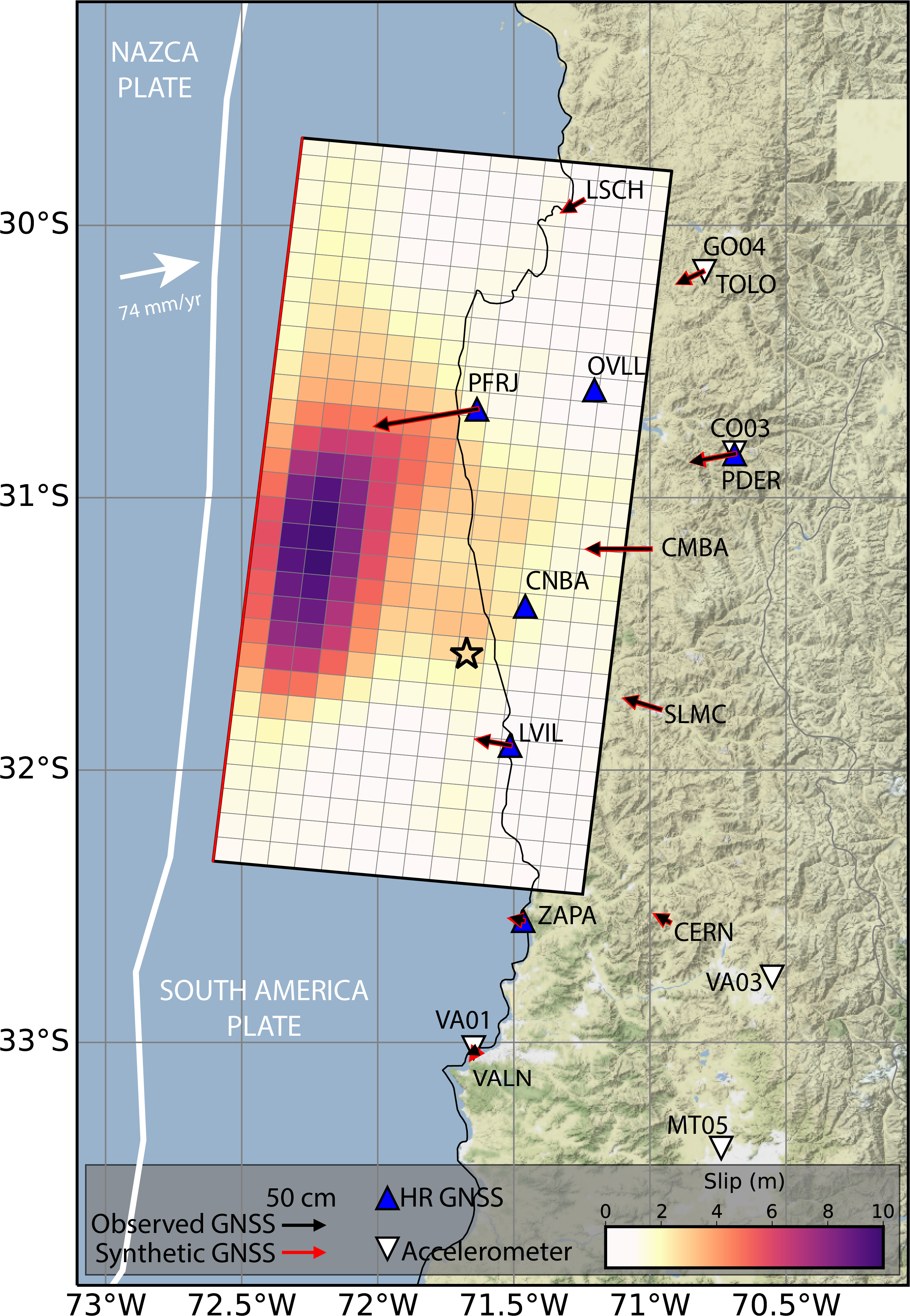
- Finite-Fault Model Maps – Map representation of the finite-fault model, in GEOJSON and PNG formats.
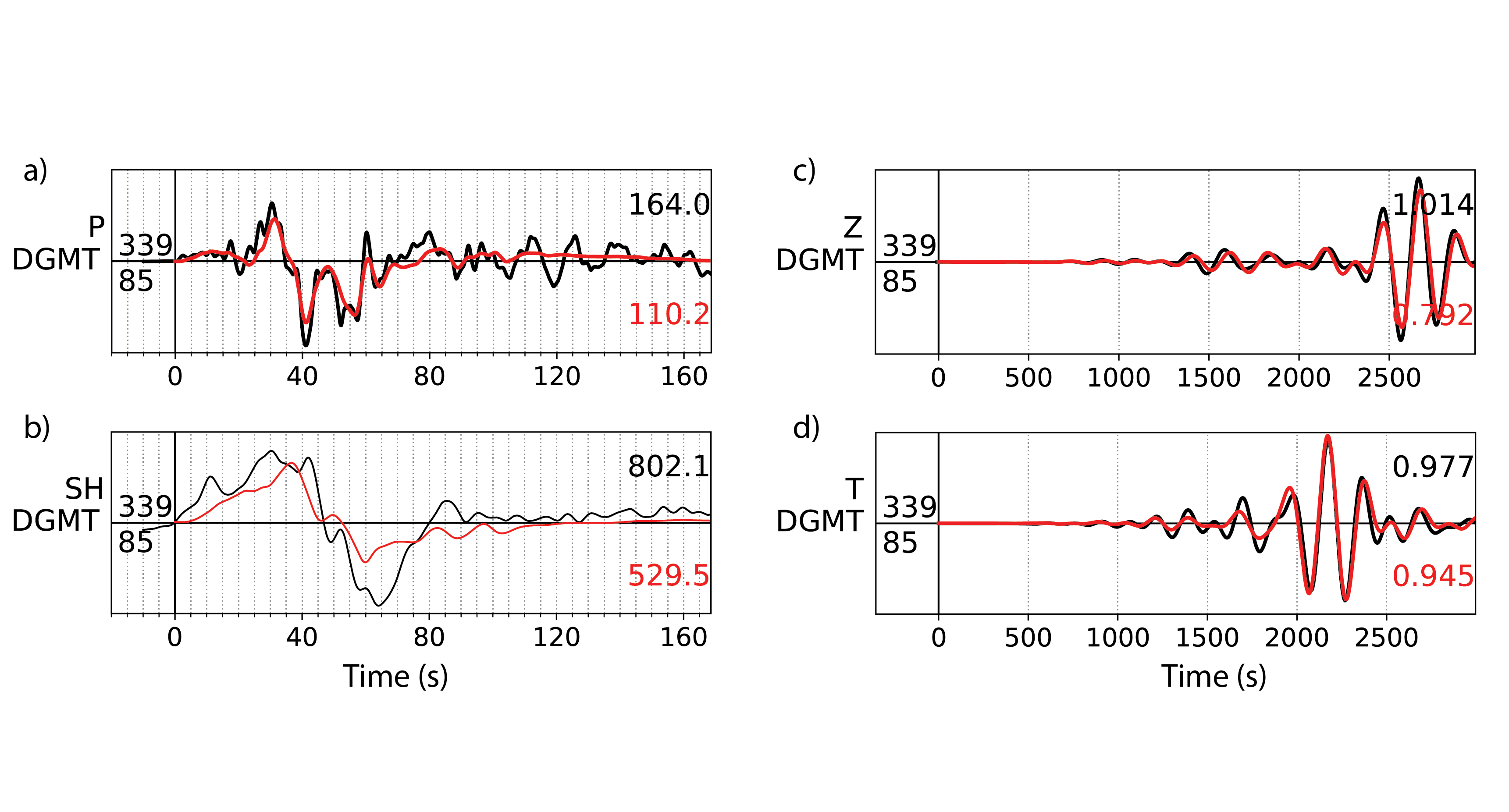
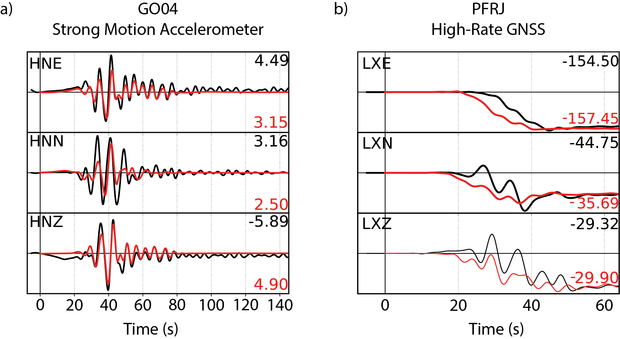
- Data and Model Fits (previously called Wave Plots) – Plots seismic and/or geodetic observations and model fits used in the inversion, in PNG format contained within a ZIP archive.
- CMT Solution - Full CMT solution for every point in the finite-fault region, in CMTSOLUTION ASCII text format (Dziewonski, Chou, & Woodhouse, 1981; http://globalcmt.org).
- Inversion Parameters – Files of inversion parameters for the finite fault, in both a static PARAM ASCII text format familiar to users of rapid NEIC fault models, and in the SRCMOD Finite Source Parameter (FSP) ASCII text format (Mai et al., 2016).
- Coulomb Input File – Input file for the Coulomb3 software package, in INP ASCII text format (Toda et al., 2011; http://earthquake.usgs.gov/research/software/coulomb/).
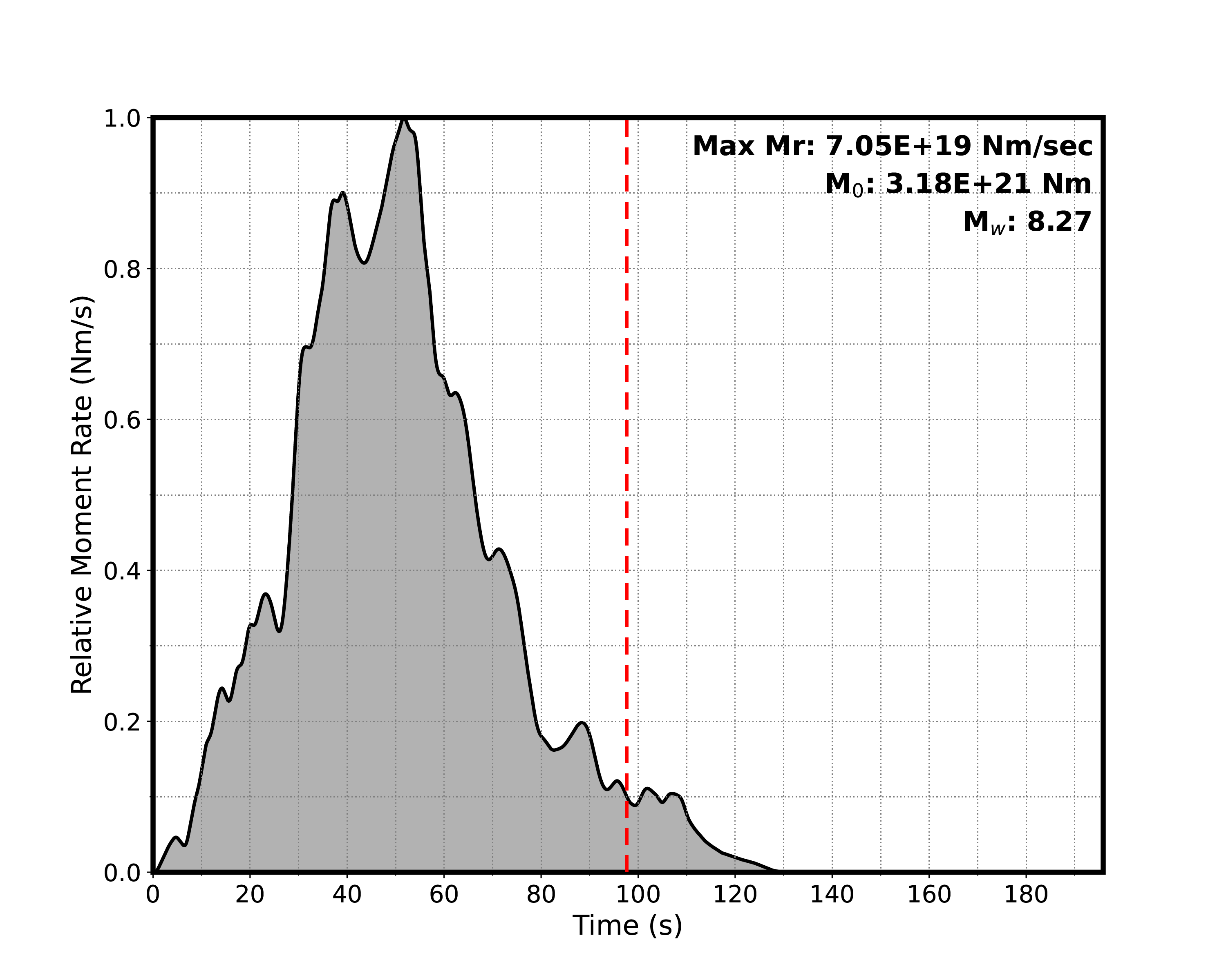
- Moment Rate Function Files – Source time function for the event, in tabular ASCII text format and plot in PNG format.
- Surface Deformation File - Surface displacement represented as three-components of predicted ground deformation, calculated using the Okada (1992) formulation, in tabular ASCII text format.
- ShakeMap Rupture Polygon File – Geometry of finite fault’s rectangular slipped area, which is used as input to ShakeMap, in ASCII text format.
- Resampled Interferogram - the resampled Interferometric Synthetic Aperture Radar (InSAR) line-of-sight surface displacement observations (available if InSAR is included in the finite-fault model), in ASCII text format, contained within a ZIP file.
Introduction to Finite-Fault Models
Earthquakes occur when there is sudden slip along a fault. Although earthquakes are most often plotted as points on a map, fault slip occurs along discrete fault surfaces that have length and width. The magnitude of an earthquake is partially determined by the area of the fault that moved and how much it moved (the slip amplitude). The seismic moment, the value seismologists use to describe the size on an earthquake, is simply the product of average slip, fault area, and shear modulus - a variable related to the strength of rock in the earthquake source region. The moment magnitude (Mw) is derived from seismic moment and is the most common type of magnitude reported for earthquakes today. The fault dimensions (length and width) and the amount of slip vary dramatically across the spectrum of earthquake magnitudes. For example, an Mw 4 earthquake fault commonly has a length of around 1 km, an Mw 7 earthquake has a length of around 40 km, and the 2004 Mw 9.1 Sumatra earthquake had a rupture length of over 1000 km.
Many factors determine the nature of shaking that is produced in the various regions around an earthquake, including the amount, rate, and location of slip. Since the shaking caused by an earthquake – and thus the impact it has on people and infrastructure – is related to the size of the area and amount of slip on the fault, constraining the slip history (what slipped and how much and when during the complete rupture) of an earthquake is an important step for earthquake response at the National Earthquake Information Center (NEIC), to improve our real time estimates of earthquake shaking (ShakeMap) and related fatalities and loses (PAGER).
The dimensions of the fault and slip amplitude along the fault that produced an earthquake can be represented in a “finite-fault model.” This model of an earthquake is generated through a “finite-fault inversion,” which uses ground motion observations of the earthquake (e.g., seismic waveforms, static displacements) to estimate where, when, and how much slip occurred. Typically, a simplified fault plane is divided into multiple sub-faults, and the inversion estimates the amount of slip on each sub-fault.
The resulting finite-fault models can be static, meaning that we estimate only the slip amplitudes and locations of slip, or kinematic, meaning that we also estimate the timing of slip. Kinematic models allow seismologists to estimate the source-time-function of an earthquake, or how seismic moment was released over the duration of the earthquake, and these models require geophysical measurements that capture how the earthquake evolved as it ruptured. In both static and kinematic models, the sum of the moment released on each subfault is equivalent to the total seismic moment, M0, of the earthquake. The earthquake magnitude, Mw, is related to seismic moment by: Mw= 2/3 (log10(M0)-9.1).
Scientific Details on Data Processing and Inversion; History of Development
Finite-fault models generated by the USGS NEIC generally employ a kinematic finite-fault inversion approach based on the method of Ji et al. (2002, 2003) and Shao et al. (2011). This approach performs finite-fault inversion by solving for the best-fitting slip amplitude, rake, rupture time, and rise time in the wavelet domain using a non-linear simulated annealing algorithm. The original inversion package was developed by Dr. Chen Ji.
Starting fault geometries are typically aligned with estimates from a Centroid Moment Tensor (CMT), either the USGS W-phase (Hayes et al., 2009) or Global CMT (Dziewonski, Chou, & Woodhouse, 1981; globalcmt.org) solution. A moment tensor solution has two potential fault plane orientations; one is the causative fault plane, and the other the auxiliary plane. The causative fault plane is the one that slipped to produce the earthquake, while the auxiliary plane is a mathematically viable solution but does not correspond to the physical event itself. In some cases, prior knowledge of the tectonic environment allows us to make an informed decision about which plane is the causative fault plane. Otherwise, both possible fault planes of the initial CMT solution are tested to account for the uncertainty regarding which plane describes the causative fault. We may then systematically vary the strike and dip of the initial geometry to test model sensitivity to these orientations or make slight variations to the fault plane orientation to fit a mapped fault geometry in the region of interest. We may further divide a favored plane into multiple fault segments if required by the data or suggested by external information.
Rupture velocity is the velocity at which the earthquake rupture front propagates across the fault plane. In the finite-fault model, rupture velocity can be fixed or allowed to vary. To account for unknown rupture characteristics, we generally test a broad distribution of fixed velocities, before settling on a final model where rupture velocity is allowed to fluctuate about a favored fixed value.
We estimate the initial fault length from empirical relationships between duration and moment (Blaser et al., 2011), scaled to length assuming a rupture velocity (generally 2.5 km/s), and multiplied by 3.3 to account for uncertainty in rupture characteristics. We model the Earth using a one-dimensional seismic velocity model based on PREM (Dziewonski & Anderson, 1981) and LITH1.0 (Pasyanos et al., 2014) global velocity models. In regions where seismic velocity structure has been well-studied, we may substitute a more detailed local velocity model from published studies.
We divide the fault plane into a series of sub-faults along the strike and dip directions. The theoretical Earth response that would be observed at a station for a unit of slip at a sub-fault is calculated using various synthetic methods (Xie and Yao, 1989; Yao and Ji, 1997; Dahlen and Tromp, 1998; Zhu and Rivera, 2002). See Ji et al. (2002) and Shao et al. (2011) for details. We use a simulated annealing approach to simultaneously solve for the slip amplitude, slip direction, rise time (the local duration of rupture), and rupture initiation time of each sub-fault, where sub-fault source time functions are modeled with an asymmetric cosine function (Ji et al., 2002, 2003).
The model is referenced spatially to the preferred hypocenter, at least initially. As with other key parameters, hypocenter location is adjusted when other information (e.g., published relocation studies) indicates a necessary recalculation.
The inversion procedure uses teleseismic body wave (P and SH observations 30-90 degrees from the source, bandpass-filtered typically between 1 and 200 s) and surface wave (Rayleigh and Love, typically bandpass-filtered between 200 and 500 s) data on a fault surface defined a priori. For each inversion, we choose to include data sampling a range of azimuths from the source, while avoiding data with small signal-to-noise ratios or poor-quality observations. Although the package is capable of jointly inverting seismic data—including both teleseismic and strong-motion recordings—as well as static displacement observations, only teleseismic data were routinely used at NEIC prior to 2021.
In adapting the package for regional applications in Chile, Koch et al. (2019) modified the heuristic rules used to automatically define the search ranges for finite-fault inversions based on the moment tensor solution, and incorporated regional strong-motion waveforms into the workflow. They also converted the codebase of the software package from Fortran 77 to Fortran 95, improving its flexibility. Goldberg et al. (2022) enabled the integration of geodetic observations into the NEIC’s near real-time finite-fault inversion framework. When available, we incorporate regional seismic and geodetic data (strong-motion accelerometer, Global Navigation Satellite Systems [GNSS], and/or Interferometric Synthetic Aperture Radar [InSAR]) into the inversion as well (Goldberg et al., 2022). Accelerometer waveforms are typically bandpass-filtered between 8 and 100 s. GNSS displacements are obtained in real-time or post-processed once final clocks and orbits become available (e.g., Melbourne et al., 2021; Bertiger et al., 2020; Herring et al., 2018).
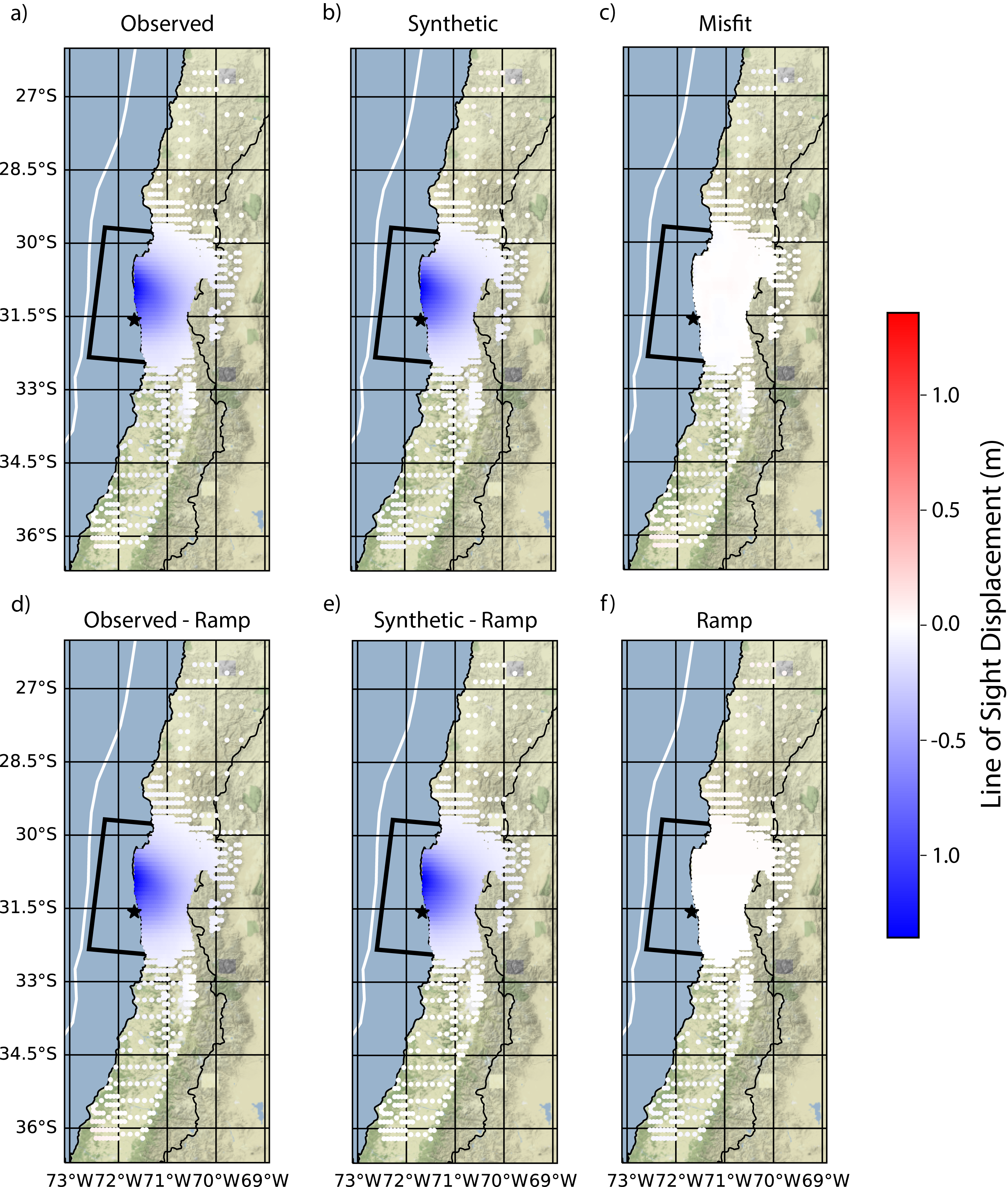
InSAR interferograms are processed with the InSAR Scientific Computing Environment (Rosen et al., 2018) package and resampled using the approach of Lohman & Simons (2005). InSAR observations may become available within hours to days after the earthquake and are generally incorporated into NEIC finite-fault models as updates in the weeks following the event. Often, long-wavelength artifacts, introduced by imprecise satellite orbit positions, result in processed interferograms showing unphysical deformation at far-field distances. This long-period signal (known as a ramp) must be disentangled from the true earthquake deformation signal. The ramp signal is solved for simultaneously during the simulated annealing procedure.
For more details on this approach and our results for past earthquakes, see Hayes (2017) and Goldberg et al. (2022a).
References
- Bertiger, W., Y. Bar-Sever, A. Dorsey, B. Haines, N. Harvey, D. Hemberger, et al. (2020). GipsyX/RTGx, a new tool set for space geodetic operations and research. Adv. Space Res., 66(3), 469–489, doi: 10.1016/ j.asr.2020.04.015.
- Blaser, L., F. Krüger, M. Ohrnberger, and F. Scherbaum (2010). Scaling relations of earthquake source parameter estimates with special focus on subduction environment. Bull. Seismol. Soc. Am., 100(6), 2914–2926, doi: 10.1785/0120100111.
- Dahlen, F. A., and J. Tromp (1998). Theoretical global seismology, Princeton University Press, Princeton, NJ.
- Dziewonski, A. M. and. D. L. Anderson (1981). Preliminary reference Earth model. Phys. Earth Planet. Int., 25(4), 297–356, doi: 10.1016/0031-9201(81)90046-7.
- Dziewonski, A. M., T.-A. Chou, and J. H. Woodhouse (1981). Determination of earthquake source parameters from waveform data for studies of global and regional seismicity. J. Geophys. Res.: Solid Earth, 86(B4), 2825–2852, doi: 10.1029/JB086iB04p02825.
- Goldberg, D. E., P. Koch, D. Melgar, S. Riquelme, and W. L. Yeck (2022a). Beyond the teleseism: Introducing regional seismic and geodetic data into routine USGS finite‐fault modeling. Seismol. Res. Lett., 93(6), 3308–3323, doi: 10.1785/0220220047.
- Goldberg, D. E., W. D. Barnhart, and B. W. Crowell (2022b). Regional and teleseismic observations for finite-fault product. U.S. Geological Survey data release, doi: 10.5066/P9ZO5FRS.
- Hayes, G. P., L. Rivera, and H. Kanamori (2009). Source inversion of the W-Phase: Real-time implementation and extension to low magnitudes. Seismol. Res. Lett., 80(5), 817–822. doi: 10.1785/gssrl.80.5.817.
- Hayes, G. P. (2017). The finite, kinematic rupture properties of great-sized earthquakes since 1990. Earth Planet. Sci. Lett., 468, 94–100, doi: 10.1016/j.epsl.2017.04.003.
- Herring, T. A., R. W. King, and S. C. McClusky (2018). Introduction to GAMIT/GLOBK, Release 10.7. Massachusetts Institute of Technology: Cambridge, Massachusetts, 54 pp.
- Ji, C., D. J. Wald, and D. V. Helmberger (2002). Source description of the 1999 Hector Mine, California earthquake; Part I: Wavelet domain inversion theory and resolution analysis. Bull. Seism. Soc. Am., 92(4), 1192–1207, doi: 10.1785/0120000916.
- Ji, C., D. V. Helmberger, D. J. Wald, and K. F. Ma (2003). Slip history and dynamic implications of the 1999 Chi-Chi, Taiwan, earthquake. J. Geophys. Res.: Solid Earth, 108(B9), 2412, doi: 10.1029/2002JB001764.
- Koch, P., F. Bravo, S. Riquelme, and J. G. Crempien (2019). Near‐real‐time finite‐fault inversions for large earthquakes in Chile using strong‐motion data. Seismol. Res. Lett., 90(5), 1971–1986, doi: 10.1785/0220180294.
- Melbourne, T. I., W. M. Szeliga, V. Marcelo Santillan, and C. W. Scrivner (2021). Global Navigational Satellite System seismic monitoring. Bull. Seismol. Soc. Am., 111(3), 1248–1262, doi: 10.1785/0120200356.
- Pasyanos, M. E., T. G. Masters, G. Laske, and Z. Ma (2014). LITHO1.0: An updated crust and lithospheric model of the Earth. J. Geophys. Res.: Solid Earth, 119(3), 2153–2173, doi: 10.1002/2013JB010626.
- Rosen, P. A., E. M. Gurrola, P. Agram, J. Cohen, M. Lavalle, et al. (2018). The InSAR scientific computing environment 3.0: A flexible framework for NISAR operational and user-led science processing, Proc. of the 2018 IEEE Int. Geoscience and Remote Sensing Symposium, 4897–4900, doi: 10.1109/IGARSS.2018.8517504.
- Shao, G. F., X. Y. Li, C. Ji, and T. Maeda (2011). Focal mechanism and slip history of the 2011 M-w 9.1 off the Pacific coast of Tohoku Earthquake, constrained with teleseismic body and surface waves, Earth Planets and Space, 63, no. 7, 559-564. doi:10.5047/eps.2011.06.028.
- Toda, S., R. S. Stein, V. Sevilgen, and J. Lin (2011). Coulomb 3.3 Graphic-rich deformation and stress-change software for earthquake, tectonic, and volcano research and teaching—user guide. U.S. Geological Survey Open-File Report 2011–1060, 63 pp., doi: 10.3133/ofr20111060.
- Xie, X.-B., and Z.-X. Yao (1989). A generalized reflection-transmission coefficient matrix method to calculate static displacement field of a stratified half-space by dislocation source, Chinese Journal of Geophysics (in Chinese), 32 (03), 270-280.
- Yao, Z. X., and C. Ji (1997). The Inversion Problem of Finite Fault Study in Time Domain, Chinese Journal of Geophysics (in Chinese), 40(05), 691-701.
- Zhu, L. and L. A. Rivera (2002). A note on the dynamic and static displacements from a point source in multilayered media. Geophys. J. Int., 148(3), 619–627, doi: 10.1046/j.1365-246X.2002.01610.x.