Two independent finite finite fault models are presented on this page. The first, using regional seismic data, comes from Doug Dreger at the Univerisity of California, Berkeley. The second, using regional GPS and InSAR data, was constructed by William Barnhart at the USGS NEIC. Both show northward-directed slip propagation. The latter is a revised distribution, having added InSAR data with more GPS time series. The two now agree more closely regarding the depth and amount of peak slip.
A preliminary finite-source slip model was obtained for the August 24, 2014 Mw6.0 West Napa earthquake by inverting seismic waveform data from 8 three-component stations of the Berkeley Digital Seismic Network (Basemap). The acceleration channels were processed by removing the mean, removing the instrument response, integrating to displacement, applying a bandpass filter between 0.02 to 1.0 Hz, and resampling the time series to 0.1 seconds/sample. Green’s functions were computed for the GIL7 velocity model (Pasyanos et al., 1996) using an FK-integration program written by Saikia. The Green’s functions where filtered with same two1pass Butterworth filter applied to the data. The finite-source code reg_inv (Dreger and Kaverina, 2000; Kaverina et al., 200 ) was used to invert for a kinematic finite-source model assuming the BSL focal mechanism (strike=155, dip=82, rake=-172).
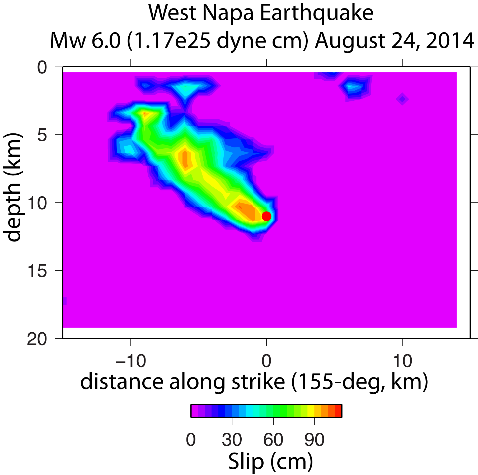
Cross-section of slip distribution. The strike direction of the fault plane is indicated below the x-axis, and the hypocenter is denoted by the red circle. Slip amplitudes are shown in color.

Comparison of regional P-waves. The data are shown in black and the synthetic seismograms are plotted in red, for each component (E-W, N-S, Z) of each station. The station name is listed at the end of each trace.

Overview of epicentral region, showing major faults in northern California (black lines), seismic station locations for data used in this inversion, and the location and faulting mechanism (beachball) for the West Napa Earthquake.

Dreger, D., and A. Kaverina (2000). Seismic remote sensing for the earthquake source process and near-source strong shaking: A case study of the October 16, 1999 Hector Mine earthquake, Geophys. Res. Lett., 27, 1941-1944.
Kaverina, A., D. Dreger, and E. Price (2002) The combined inversion of seismic and geodetic data for the source process of the 16 October 1999 M (sub w) 7.1 Hector Mine, California, Earthquake, Bull. Seism. Soc. Am., vol.92, no.4, pp.1266-1280.
Pasyanos, M. E., D. S. Dreger, and B. Romanowicz (1996), Towards Real-Time Determination of Regional Moment Tensors, Bull. Seism. Soc. Am., 86, 1255-1269.
This updated slip distribution is inverted from 56 continuous GPS time series processed by the USGS to determine horizontal static offsets at the event origin time and associated error bounds. We also surface displacements from a coseismic interferogram produced by the JPL/ARIA group (2014/07/26-2014/08/27). Inversion of faulting parameters followed the methodology of Barnhart et al. [2014] and Barnhart and Lohman [2010], in which we inverted for fault location, geometry (strike, dip), and location and magnitude of slip. Slip direction was fixed to 178° (right-lateral slip). No CMT or epicentral information was used to pre-condition the inversion. The different sizes of fault patches are automatically defined and result from variable resolution of the inversion with respect to depth and data quality.
After comparing GPS and InSAR displacement fits, we find that the northeast-dipping nodal plane (strike=341 deg., dip=80 deg, rake = 176 deg.) fits the observations best. This is in strong agreement with seismic moment tensors and focal mechanisms. Likewise, the NoCal CMT epicenter is within 100 m of the modeled fault plane. The enhanced resolution afforded by the InSAR observations shows a slip centroid centered near 5 km depth, with some slip extending to the surface, in accordance with field observations. The resulting magnitude of the slip distribution is Mw6.05.
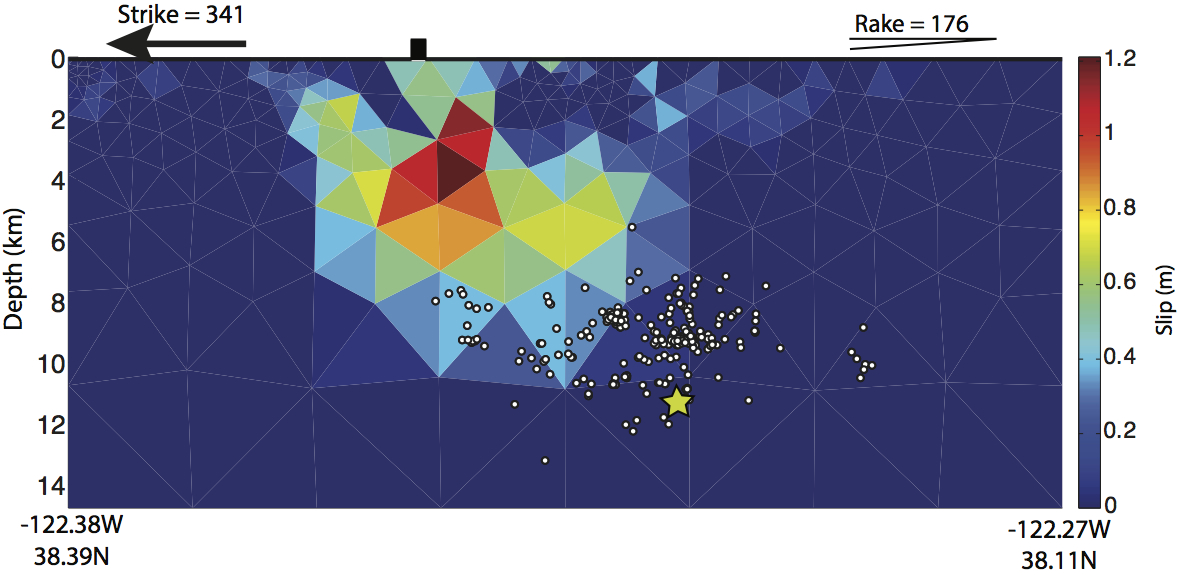
Cross-section of slip distribution. The strike direction of the fault plane is indicated by the black arrow, and the hypocenter is denoted by the yellow star. Slip amplitudes are shown in color, and motion of the western wall (hanging wall) relative to the ground surface and footwall of the fault is indicated by the black rake reference arrow. White dots are relocated aftershocks provided by J. Hardebeck, and the rectangle on the fault trace indicates the location of maximum mapped surface displacements from field observations (B. Brooks, USGS).

GPS displacements and associated error ellipses are shown in black, and surface displacements predicted by the slip distribution are shown in red. The fault location and slip distribution are plotted on top.

Resampled InSAR displacements and displacements predicted by the slip inversion. The fault location and slip distribution are plotted on top.
| SUBFAULT FORMAT | COULOMB INPUT FORMAT | GOOGLE KMZ FORMAT |
This work is supported by the National Earthquake Information Center (NEIC) of United States Geological Survey. This web page is built and maintained by Dr. G. Hayes at the NEIC.